
Capturing the Data (continued)
As mentioned earlier, the LM-1 has six built-in channels,
one of which is pre-populated by the wide-band oxygen sensor.
In order to utilize the other channels we used the LMA-3
"Aux Box" device. This device is really the core
tool for data-logging with the LM-1 because it comes with
several built-in sensors and functions. For instance, the
built in 3-bar MAP sensor simplifies measuring boost pressure.
We simply T'd the vacuum line from our boost gauge and connected
to the port on the LMA-3. The unit also has a built in rpm
converter, so we just tapped in to the MSD tach-ouput lead.
We were also interested in monitoring fuel pressure. For
this we replaced the analog pressure gauge in the fuel line
with a pressure transducer. This sensor sends a linear voltage
signal, 0.5V for 0 psi to 4.5V for 100 psi. The steps below
show how to hook up the LM1 and LMA-3 and begin logging
data.

 The first step is to hook up the auxiliary unit. We
connected a vacuum line to the built-in MAP sensor on
the LMA-3 to measure boost pressure. The terminals on
the left are for the other channels. Channel 1 is default
for RPM input, so that is where we connected our tach
lead from the MSD unit. We followed the instructions
to set the unit for 8 cylinders. The unit should be
mounted inside the cabin, and level if using the built-in
accelerometer.
The first step is to hook up the auxiliary unit. We
connected a vacuum line to the built-in MAP sensor on
the LMA-3 to measure boost pressure. The terminals on
the left are for the other channels. Channel 1 is default
for RPM input, so that is where we connected our tach
lead from the MSD unit. We followed the instructions
to set the unit for 8 cylinders. The unit should be
mounted inside the cabin, and level if using the built-in
accelerometer. |
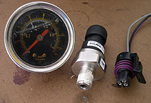
 Sensors, such as this 0-100psi pressure transducer,
are used to send data to the LMA-3 in 0-5V signals.
The sensor has three wires (5V input, ground, and
0-5V output.) The LMA-3 has a convenient 5V output
(bottom terminal) so you do not have to create one.
The output lead from the sensor connects to an open
channel on the LMA-3. Sensors like these are found
on many Ford and GM cars, and also in aftermarket
products like Autometer electric gauges.
Sensors, such as this 0-100psi pressure transducer,
are used to send data to the LMA-3 in 0-5V signals.
The sensor has three wires (5V input, ground, and
0-5V output.) The LMA-3 has a convenient 5V output
(bottom terminal) so you do not have to create one.
The output lead from the sensor connects to an open
channel on the LMA-3. Sensors like these are found
on many Ford and GM cars, and also in aftermarket
products like Autometer electric gauges.
|

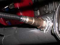
 The
next step is to install the wide-band O2 sensor. Either
weld in a bung (see side bar) or alternatively use an
exhaust
clamp from Innovate, as seen here on our '01. Note
that for the sensor to read accurately you must locate
it before the catalytic converters, or as in our case
have no converters to deal with. Because condensation
in the pipe can damage the sensor it is good practice
to only install the sensor when you plan to data log. The
next step is to install the wide-band O2 sensor. Either
weld in a bung (see side bar) or alternatively use an
exhaust
clamp from Innovate, as seen here on our '01. Note
that for the sensor to read accurately you must locate
it before the catalytic converters, or as in our case
have no converters to deal with. Because condensation
in the pipe can damage the sensor it is good practice
to only install the sensor when you plan to data log. |

 Make the connections to the LM-1. The unit comes with
a cigarette lighter power adapter, this must be connected
as it operates the O2 sensor heater. The O2 sensor cable
plugs in to the port marked "sensor". The
auxiliary unit (LMA-2 or LMA-3) connects to "Aux
In". The "Serial Port" connection is
used to connect to a PC, and the "Analog Out"
port can be used to send data to another system or external
A/F gauge.
Make the connections to the LM-1. The unit comes with
a cigarette lighter power adapter, this must be connected
as it operates the O2 sensor heater. The O2 sensor cable
plugs in to the port marked "sensor". The
auxiliary unit (LMA-2 or LMA-3) connects to "Aux
In". The "Serial Port" connection is
used to connect to a PC, and the "Analog Out"
port can be used to send data to another system or external
A/F gauge. |

 Once the connections are made, turn the unit on. The
very first time the unit is powered it will perform
a calibration for the sensor. After that you can start
the motor and the unit. The LM-1 LCD will display a
"warm up mode" for about 20 seconds then it
should display the air/fuel ratio of the exhaust or
20.9% oxygen if the sensor is in free air. A calibrate
button is provided in order to calibrate the unit due
to air density changes.
Once the connections are made, turn the unit on. The
very first time the unit is powered it will perform
a calibration for the sensor. After that you can start
the motor and the unit. The LM-1 LCD will display a
"warm up mode" for about 20 seconds then it
should display the air/fuel ratio of the exhaust or
20.9% oxygen if the sensor is in free air. A calibrate
button is provided in order to calibrate the unit due
to air density changes. |
 If you have a laptop you can view the data in real time
using Logworks. Because voltage itself is not terribly
meaningful you can configure each channel to what the
voltage converts to for your particular sensor. AFR,
RPM, and the built in sensors on the LMA-3 come pre-configured
for ease. When ready to log data, hit the red record
button. Press the button again when you want to stop
recording.
If you have a laptop you can view the data in real time
using Logworks. Because voltage itself is not terribly
meaningful you can configure each channel to what the
voltage converts to for your particular sensor. AFR,
RPM, and the built in sensors on the LMA-3 come pre-configured
for ease. When ready to log data, hit the red record
button. Press the button again when you want to stop
recording. |
Analyzing the Data
We went out to our favorite
stretch of desolate road and made a half-dozen runs in various
gears, full and part-throttle. The nice thing about the
LM-1 is that unlike other tools or track testing, you do
not have to run through all the gears or a full quarter
mile to get results. We got the car up to a good cruise
rpm hit the red "record" button on the box and
then stabbed the throttle. The red button is pressed again
to stop recording the session. The LM-1 will assign a sequential
file name to each session until the 44 minute storage capacity
is used up. Then you must download the data to your PC to
clear the memory.
We opened up the LogWorks program to review the sessions.
Here we can not only analyze the data in more ways then
a ballot recount in Florida, but we can also replay the
session and watch all the gauge needles dance around as
they did during the drive. Below is a screenshot of what
one of our runs looked like while under boost. Each color
trace on the graph corresponds to a data channel. We were
logging on 4 channels: AFR, RPM, Fuel pressure, and boost
pressure (MAP). We turned off the remaining two channels
because we were not logging data on them.
 What our data shows is that as the
supercharger builds boost (blue line) the air/fuel ratio goes
into dangerously lean territory (pink line.) Note that we
have set the Y-axis to show air/fuel ratio (AFR) units. This
can be changed to show the units for any of the channels.
The X-axis always shows time in seconds. We have set a call-out
just past the 8 second mark which lists the data for all channels
at the point. Note the AFR is at 17:1 when boost pressure
is at 4psi. Looking at the fuel pressure (green line) we see
the likely source of the problem - not enough fuel. Baseline
fuel pressure without boost is 10psi. Our boost referenced
fuel pump should be rising 1psi above baseline for each 1psi
rise in boost. We would expect 14psi or more of fuel pressure,
which we are not quite achieving. Another observation is the
major fluctuation in fuel pressure as boost comes on. With
this data we are able to conclude with fair certainty that
fuel starvation is the problem, and the next step will be
to upgrade the fuel system. We can also view and sort the
data in several different ways (see side bar) to get the information
we need.
What our data shows is that as the
supercharger builds boost (blue line) the air/fuel ratio goes
into dangerously lean territory (pink line.) Note that we
have set the Y-axis to show air/fuel ratio (AFR) units. This
can be changed to show the units for any of the channels.
The X-axis always shows time in seconds. We have set a call-out
just past the 8 second mark which lists the data for all channels
at the point. Note the AFR is at 17:1 when boost pressure
is at 4psi. Looking at the fuel pressure (green line) we see
the likely source of the problem - not enough fuel. Baseline
fuel pressure without boost is 10psi. Our boost referenced
fuel pump should be rising 1psi above baseline for each 1psi
rise in boost. We would expect 14psi or more of fuel pressure,
which we are not quite achieving. Another observation is the
major fluctuation in fuel pressure as boost comes on. With
this data we are able to conclude with fair certainty that
fuel starvation is the problem, and the next step will be
to upgrade the fuel system. We can also view and sort the
data in several different ways (see side bar) to get the information
we need.
Endless Capability
Air/fuel ratio, rpm and fuel pressure are very fundamental
tuning parameters. However they are just scratching the surface
of the tuning capabilities with data logging. The possibilities
for what you can monitor are virtually endless. One need not
look further than many late model vehicles, which have sensors
to monitor all sorts of engine and vehicle conditions. Chances
are there is a 0-5V sensor out there that can measure whatever
it is you are interested in logging. If there isn't, then
someone on the Innovate
Support Forums has likely put together a circuit diagram
for how to build the sensor using Radio Shack parts. In any
case the exciting thing about the LM-1 is that there is a
rapidly growing online user community from which you can learn,
share ideas, and get technical help. In fact, the LM-1's principal
engineer, Klaus Allmendinger, is routinely on the forums providing
technical assistance.
A few ideas we're starting to play around with, and which
you will see in future articles, are using the LMA-3's internal
G-force sensor to measure rate of acceleration. We can make
changes to the engine or vehicle, log a run, and then using
LogWorks overlay function to compare before and after G-force
data. In this way we are not slaves to the track or dyno for
determining performance improvements.  |
| |
|
| |
|
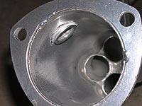
Installing an O2 Sensor Bung
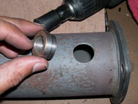
Using a hole saw we cut out a hole at the end of the
header collector. Before drilling ensure the sensor
or wiring will not interfere with the frame or other
parts under the car. We then welded the bung into place.
The bung (and plug) are included in the kit. In a pinch
you can even use an 18mm nut. |
The O2 sensor is best installed in the 3 or 9 o'clock
position. Installing too close to the primary tubes
can result in poor sensor performance due to overheating
and cylinder pulses. The sensor can be installed as
far back as the tail pipe, so long as the exhaust system
is free from leaks. |

Our headers were beginning to develop surface rust,
and were looking generally pretty ragged. Rather than
fork out for another $400 for a set of Hooker SuperComps,
which would eventually turn ugly too, we sent the headers
to Jet-Hot
for coating. |
The results are stunning. The Jet-Hot Sterling coating
reaches the inside of the header as well. Using a thermocouple
we measured a 80°F reduction in surface temperature
of the primary tubes. Look for more in an upcoming article. |
|
|
Great
View
There are several ways to sort and
view the data from your logging session.
The Statistics plot is useful for viewing
how often an event occurs. You can select the section of time
where you want to perform the analysis. In this case we see
that our fuel pressure is on average 12 psi +/- 2. |
| |
The X-Y plot lets you view data from
a channel in the context of another channel. In this case
we have boost/vacuum pressure on the x-axis and fuel on the
Y-axis. We see that at cruise fuel pressure is between 10-12psi.
Under boost pressure goes only to 12-14psi, however note all
the erratic data points, some as low as 8 psi. |
| |
The Chart view enables you to create
a 3D sorting of the data. Here we are looking MAP sensor data
(vacuum/boost) over rpm and air/fuel ratio. We can see that
lean conditions correspond to a rise in rpm and boost pressure. |
| |
|
Sources:
Innovate! Technology, Inc.
27122A Paseo Espada #904
San Juan Capistrano
California 92675
Tel : 949.388.4442
www.innovatemotorsports.com |
|
|